ds4n6_lib And Binder, A Quick Way To Try The New Library
 | [22/04/21] April 22, 2021 David Contreras - One eSecurity Twitter: dcontrerasDS - LinkedIn: David Contreras |
For the Impatient…
If you just want to try the Jupyter notebooks even before reading this blog post, you can click this Binder button  , wait a few (2-5) minutes for the environment to be created, open a notebook and run all cells via: Cell → Run All
What is this post about?
As a part of the ds4n6_lib release, we have created a bunch of analysis notebooks integrated with different tools and artifacts that you can download from GitHub. These notebooks are prepared to load the needed libraries, the evidence and run some DS4N6 functions to show you how to use them for your investigations. We will be uploading more notebooks, but at this moment the available ones are:
In this post we want to explain you how to try the notebooks and the library in less than 15 minutes using some of these notebooks.
Starting with Binder
There are many different tools that can be used to load and try Jupyter notebooks in the cloud, such as Binder, Google Colab or Kaggle. In this entry we are going to use Binder, explaining how to get started with the new ds4n6_lib.
Binder is one of the easiest ways to work with Jupyter notebooks. There is no need to create an account and just selecting the GitHub project you want to load, you will have a new and ready-to-use environment to start working in a few minutes. Binder will take care of the dependencies and everything you need. If you want to try the ds4n6_lib library in Binder, just click the following button 
Let's get started with Jupyter!
As you can see in the screenshot, once the environment has been loaded, we have a couple of notebooks that are ready to be used. For this entry, we are starting with the musctf19-plaso.ipynb notebook.
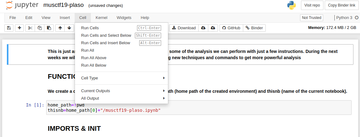
The first thing you need to do is to open the notebook with a click and run all cells as showed in the next screenshot. This will run the whole notebook, loading all the libraries, downloading the evidence and preparing the analysis.
Reading data
As you already have a little explanation of what each cell does in the notebook, here we will explain some functions in more detail. To know how the functions work, we recommend you to read this post:
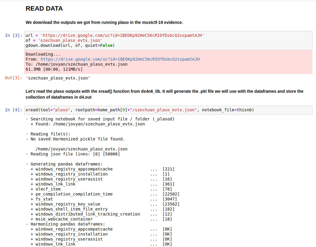
After loading all the libraries, the first thing we need to do is to read the data as you can see in the picture above. We will download the outputs we got running plaso in the evidence to use them for the analysis. We do it via gdown functions. If you have your own plaso outputs in json format, you can change the URL ID and download the yours. Once we have the data, it's time to read, and we do it with xread, which comes from ds4n6_lib. It allows to read the data from different tools, performing two action:
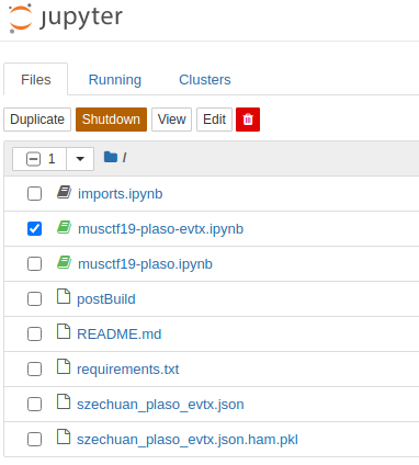
- It creates an harmonized pickle with all the information (you will notice szechuan_plaso_evtx.json.ham.pkl is in you home). This .pkl file is the one used to read the data in a very fast way from now. You can learn more about .pkl files here
- It creates a collection of dataframes, what we usually name as a dataframes dictionary, storing it in the d4.out variable. We will talk about some concepts, as dictionaries, in future posts, but to understand what is happening here we are getting one dataframe per artifact parsed with plaso (in the screenshot below, each row when generating pandas dataframes). It means we will have one dataframe for windows_registry_appcompatcache, another one for windows_registry_installation, etc. All these dataframes are stored in the same variable, d4.out, and this variable is what we call dictionary of dataframes.
Now let's take a look at the home folder, you will notice a couple of new files: szechuan_plaso_evtx.json file and szechuan_plaso_evtx.json.ham.pkl.
First analysis
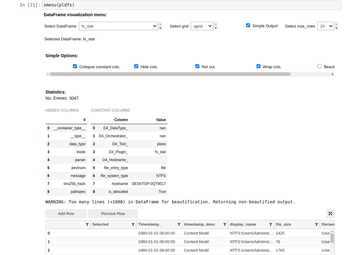
In the xmenu, we will be able to display the data we have already read. Once we select the dataframe or the column we want to analyze, we can select different grids to filter or perform different actions. If you get a dataframe that is interesting for further analysis, you can click in the export button you have below the table. It will export the displayed dataframe to the d4.out variable as a dataframe
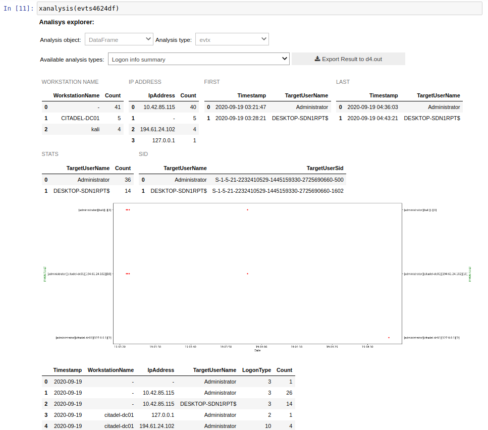
The last cell is xanalysis. This function, as xmenu, is a powerful and cross function for all the dataframes regardless where they come from. As we have much more interesting analysis for Windows Events, we will use the second notebook provided for this demo: musctf19-plaso-evtx
First of all, let's run all the cells in the same way as before, and let's move to the xanalysis() function.
As you can see, to perform a new analysis you only have to select some parameters depending on the argument you pass to the function. In this case, as we are analyzing a dataframe, we only have to select the analysis type we want to perform. xanalysis function will show you the available analysis for the dataframe type that you are passing. In this case, as we are using a dataframe with Windows Events, xanalysis shows the two available analysis for this artifact. By selecting the Logon info summary analysis, we will immediately get a new analysis with statistics about all the logins and a graph indicating some possible anomalies. In a further post we will explain the Windows Events analysis tool developed with ds4n6_lib and these analysis in a deeper way.
Now it is time for you to play with the dataframes and analysis. Enjoy!
A couple of extra tips
Just a couple of tips about the use of Binder:
- If you are trying a dataframe with several columns, you will notice it is not very comfortable to analyze it in the small area you get. With the qgrid shape, a click in the button you have just in the up-right corner of the dataframe will open it in full screen
- If you want to try different notebooks, one tip: binder gives you 2GB of memory for all the kernels, so don't forget to restart the kernel when you are done with a notebook.
To finish this entry, I would like to remind you that in this post, we have loaded just a few data to show you how to use the new ds4n6_lib but, remember, the power of the use of DS for the analysis is that you can do the same process with millions of records from many computers, performing this analysis in just a few minutes. Welcome to DS4N6!


